Installation
First, setup the prerequest for PyQMRI:
[ ]:
!apt-get update
!apt-get install libclfft-dev -y
Hit:1 https://cloud.r-project.org/bin/linux/ubuntu bionic-cran40/ InRelease
Ign:2 https://developer.download.nvidia.com/compute/cuda/repos/ubuntu1804/x86_64  InRelease
Hit:3 http://security.ubuntu.com/ubuntu bionic-security InRelease
Ign:4 https://developer.download.nvidia.com/compute/machine-learning/repos/ubuntu1804/x86_64  InRelease
Hit:5 https://developer.download.nvidia.com/compute/cuda/repos/ubuntu1804/x86_64  Release
Hit:6 https://developer.download.nvidia.com/compute/machine-learning/repos/ubuntu1804/x86_64  Release
Hit:7 http://archive.ubuntu.com/ubuntu bionic InRelease
Hit:8 http://ppa.launchpad.net/c2d4u.team/c2d4u4.0+/ubuntu bionic InRelease
Hit:9 http://archive.ubuntu.com/ubuntu bionic-updates InRelease
Hit:10 http://archive.ubuntu.com/ubuntu bionic-backports InRelease
Hit:11 http://ppa.launchpad.net/graphics-drivers/ppa/ubuntu bionic InRelease
Reading package lists... Done
Reading package lists... Done
Building dependency tree
Reading state information... Done
libclfft-dev is already the newest version (2.12.2-1build2).
0 upgraded, 0 newly installed, 0 to remove and 31 not upgraded.
[ ]:
!git clone https://github.com/geggo/gpyfft.git
fatal: destination path 'gpyfft' already exists and is not an empty directory.
[ ]:
!pip install gpyfft/.
Processing ./gpyfft
Requirement already satisfied: numpy in /usr/local/lib/python3.6/dist-packages (from gpyfft==0.7.3) (1.18.5)
Requirement already satisfied: pyopencl in /usr/local/lib/python3.6/dist-packages (from gpyfft==0.7.3) (2020.2.2)
Requirement already satisfied: appdirs>=1.4.0 in /usr/local/lib/python3.6/dist-packages (from pyopencl->gpyfft==0.7.3) (1.4.4)
Requirement already satisfied: decorator>=3.2.0 in /usr/local/lib/python3.6/dist-packages (from pyopencl->gpyfft==0.7.3) (4.4.2)
Requirement already satisfied: pytools>=2017.6 in /usr/local/lib/python3.6/dist-packages (from pyopencl->gpyfft==0.7.3) (2020.4.3)
Requirement already satisfied: dataclasses>=0.7; python_version <= "3.6" in /usr/local/lib/python3.6/dist-packages (from pytools>=2017.6->pyopencl->gpyfft==0.7.3) (0.7)
Requirement already satisfied: six>=1.8.0 in /usr/local/lib/python3.6/dist-packages (from pytools>=2017.6->pyopencl->gpyfft==0.7.3) (1.15.0)
Building wheels for collected packages: gpyfft
  Building wheel for gpyfft (setup.py) ... done
  Created wheel for gpyfft: filename=gpyfft-0.7.3-cp36-cp36m-linux_x86_64.whl size=367757 sha256=609c21b4b3d4d1516f80522ca6085730f8f1b3ac6831e3e50ef0ae94f0c4ec8d
  Stored in directory: /tmp/pip-ephem-wheel-cache-hgbwtlsh/wheels/59/8e/ab/202c7b2221f0b7acf0f9b0f7ce9c9c7697830acdd5bd6d7aa5
Successfully built gpyfft
Installing collected packages: gpyfft
  Found existing installation: gpyfft 0.7.3
    Uninstalling gpyfft-0.7.3:
      Successfully uninstalled gpyfft-0.7.3
Successfully installed gpyfft-0.7.3
After the successfull installation of the prerequests, we can install PyQMRI itself:
[ ]:
!pip install pyqmri
Requirement already satisfied: pyqmri in /usr/local/lib/python3.6/dist-packages (0.3.2.3)
Requirement already satisfied: matplotlib in /usr/local/lib/python3.6/dist-packages (from pyqmri) (3.2.2)
Requirement already satisfied: pyfftw in /usr/local/lib/python3.6/dist-packages (from pyqmri) (0.12.0)
Requirement already satisfied: h5py in /usr/local/lib/python3.6/dist-packages (from pyqmri) (2.10.0)
Requirement already satisfied: ipyparallel in /usr/local/lib/python3.6/dist-packages (from pyqmri) (6.3.0)
Requirement already satisfied: cython in /usr/local/lib/python3.6/dist-packages (from pyqmri) (0.29.21)
Requirement already satisfied: numpy in /usr/local/lib/python3.6/dist-packages (from pyqmri) (1.18.5)
Requirement already satisfied: numexpr in /usr/local/lib/python3.6/dist-packages (from pyqmri) (2.7.1)
Requirement already satisfied: pyqt5 in /usr/local/lib/python3.6/dist-packages (from pyqmri) (5.15.1)
Requirement already satisfied: mako in /usr/local/lib/python3.6/dist-packages (from pyqmri) (1.1.3)
Requirement already satisfied: sympy>=1.6.2 in /usr/local/lib/python3.6/dist-packages (from pyqmri) (1.6.2)
Requirement already satisfied: pyopencl in /usr/local/lib/python3.6/dist-packages (from pyqmri) (2020.2.2)
Requirement already satisfied: cycler>=0.10 in /usr/local/lib/python3.6/dist-packages (from matplotlib->pyqmri) (0.10.0)
Requirement already satisfied: python-dateutil>=2.1 in /usr/local/lib/python3.6/dist-packages (from matplotlib->pyqmri) (2.8.1)
Requirement already satisfied: pyparsing!=2.0.4,!=2.1.2,!=2.1.6,>=2.0.1 in /usr/local/lib/python3.6/dist-packages (from matplotlib->pyqmri) (2.4.7)
Requirement already satisfied: kiwisolver>=1.0.1 in /usr/local/lib/python3.6/dist-packages (from matplotlib->pyqmri) (1.2.0)
Requirement already satisfied: six in /usr/local/lib/python3.6/dist-packages (from h5py->pyqmri) (1.15.0)
Requirement already satisfied: traitlets>=4.3 in /usr/local/lib/python3.6/dist-packages (from ipyparallel->pyqmri) (4.3.3)
Requirement already satisfied: ipykernel>=4.4 in /usr/local/lib/python3.6/dist-packages (from ipyparallel->pyqmri) (4.10.1)
Requirement already satisfied: jupyter-client in /usr/local/lib/python3.6/dist-packages (from ipyparallel->pyqmri) (5.3.5)
Requirement already satisfied: tornado>=4 in /usr/local/lib/python3.6/dist-packages (from ipyparallel->pyqmri) (5.1.1)
Requirement already satisfied: ipython-genutils in /usr/local/lib/python3.6/dist-packages (from ipyparallel->pyqmri) (0.2.0)
Requirement already satisfied: pyzmq>=13 in /usr/local/lib/python3.6/dist-packages (from ipyparallel->pyqmri) (19.0.2)
Requirement already satisfied: ipython>=4 in /usr/local/lib/python3.6/dist-packages (from ipyparallel->pyqmri) (5.5.0)
Requirement already satisfied: decorator in /usr/local/lib/python3.6/dist-packages (from ipyparallel->pyqmri) (4.4.2)
Requirement already satisfied: PyQt5-sip<13,>=12.8 in /usr/local/lib/python3.6/dist-packages (from pyqt5->pyqmri) (12.8.1)
Requirement already satisfied: MarkupSafe>=0.9.2 in /usr/local/lib/python3.6/dist-packages (from mako->pyqmri) (1.1.1)
Requirement already satisfied: mpmath>=0.19 in /usr/local/lib/python3.6/dist-packages (from sympy>=1.6.2->pyqmri) (1.1.0)
Requirement already satisfied: pytools>=2017.6 in /usr/local/lib/python3.6/dist-packages (from pyopencl->pyqmri) (2020.4.3)
Requirement already satisfied: appdirs>=1.4.0 in /usr/local/lib/python3.6/dist-packages (from pyopencl->pyqmri) (1.4.4)
Requirement already satisfied: jupyter-core>=4.6.0 in /usr/local/lib/python3.6/dist-packages (from jupyter-client->ipyparallel->pyqmri) (4.6.3)
Requirement already satisfied: setuptools>=18.5 in /usr/local/lib/python3.6/dist-packages (from ipython>=4->ipyparallel->pyqmri) (50.3.2)
Requirement already satisfied: pygments in /usr/local/lib/python3.6/dist-packages (from ipython>=4->ipyparallel->pyqmri) (2.6.1)
Requirement already satisfied: pickleshare in /usr/local/lib/python3.6/dist-packages (from ipython>=4->ipyparallel->pyqmri) (0.7.5)
Requirement already satisfied: pexpect; sys_platform != "win32" in /usr/local/lib/python3.6/dist-packages (from ipython>=4->ipyparallel->pyqmri) (4.8.0)
Requirement already satisfied: prompt-toolkit<2.0.0,>=1.0.4 in /usr/local/lib/python3.6/dist-packages (from ipython>=4->ipyparallel->pyqmri) (1.0.18)
Requirement already satisfied: simplegeneric>0.8 in /usr/local/lib/python3.6/dist-packages (from ipython>=4->ipyparallel->pyqmri) (0.8.1)
Requirement already satisfied: dataclasses>=0.7; python_version <= "3.6" in /usr/local/lib/python3.6/dist-packages (from pytools>=2017.6->pyopencl->pyqmri) (0.7)
Requirement already satisfied: ptyprocess>=0.5 in /usr/local/lib/python3.6/dist-packages (from pexpect; sys_platform != "win32"->ipython>=4->ipyparallel->pyqmri) (0.6.0)
Requirement already satisfied: wcwidth in /usr/local/lib/python3.6/dist-packages (from prompt-toolkit<2.0.0,>=1.0.4->ipython>=4->ipyparallel->pyqmri) (0.2.5)
And that was it already. PyQMRI is installed on the system. # Example data Next, lets have a look at some example data to run the reconstruction with. We will use radially acquired VFA data consisting of 10 flip angles (Scans) and 34 radial projections each.
Downloading this file might take some time, depending on the speed of the internet connection.
[ ]:
import os
%cd sample_data/
if not os.path.isfile("23052018_VFA_34.h5"):
  !wget https://zenodo.org/record/1410918/files/23052018_VFA_34.h5
%cd ..
/content/sample_data
--2020-11-03 14:46:43--  https://zenodo.org/record/1410918/files/23052018_VFA_34.h5
Resolving zenodo.org (zenodo.org)... 137.138.76.77
Connecting to zenodo.org (zenodo.org)|137.138.76.77|:443... connected.
HTTP request sent, awaiting response... 200 OK
Length: 1688253784 (1.6G) [application/octet-stream]
Saving to: ‘23052018_VFA_34.h5’

23052018_VFA_34.h5  100%[===================>]   1.57G  9.43MB/s    in 3m 0s

2020-11-03 14:49:44 (8.93 MB/s) - ‘23052018_VFA_34.h5’ saved [1688253784/1688253784]

/content
Ok so we have some data now. Lets explore what is inside of this .h5 file:
[ ]:
import h5py

with h5py.File('sample_data/23052018_VFA_34.h5', 'r') as file:
  print("Data content: " + str(file.keys()))
  print("Additional (sequence related) attributes: " + str(file.attrs.keys()))
Data content: <KeysViewHDF5 ['Coils', 'dcf', 'fa_corr', 'imag_dat', 'imag_traj', 'real_dat', 'real_traj']>
Additional (sequence related) attributes: <KeysViewHDF5 ['TR', 'data_normalized_with_dcf', 'flip_angle(s)', 'image_dimensions']>
Now we know what to expect. This File reflects the rawdata and necessary attributes to start the reconstruction/fitting process of PyQMRI.
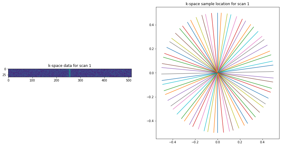
The data was acquired in a non-Cartesian fashion, as can be seen from the fact that *_traj* entries exists in the data itself.
Visualizing the data and trajectory gives:
[ ]:
import matplotlib.pyplot as plt
import numpy as np

with h5py.File('sample_data/23052018_VFA_34.h5', 'r') as file:
  data = file["real_dat"][()] + 1j* file["imag_dat"][()]
  trajectory = file["real_traj"][()] + 1j* file["imag_traj"][()]

fig = plt.figure(figsize=(16,8))
ax = fig.add_subplot(121)
ax.imshow(np.abs(data[0,0,0]))
tmp = plt.title("k-space data for scan 1")
ax = fig.add_subplot(122)
trajectory.shape
plot = ax.plot(trajectory[0].real.T, trajectory[0].imag.T)
tmp = plt.title("k-space sample location for scan 1")
As this file served as input for an older version we need to deleted to old coil sensitivity profiles Coils because they will have a wrong orientation.
[ ]:
with h5py.File('sample_data/23052018_VFA_34.h5', 'r+') as file:
  del file["Coils"]
Lets check if that was succesfull:
[ ]:
with h5py.File('sample_data/23052018_VFA_34.h5', 'r') as file:
  print("Data content: " + str(file.keys()))
  print("Additional (sequence related) attributes: " + str(file.attrs.keys()))
Data content: <KeysViewHDF5 ['dcf', 'fa_corr', 'imag_dat', 'imag_traj', 'real_dat', 'real_traj']>
Additional (sequence related) attributes: <KeysViewHDF5 ['TR', 'data_normalized_with_dcf', 'flip_angle(s)', 'image_dimensions']>
Perfect. The old coil sensitivity maps are gone and we are ready to start the fitting. As a quick side note, the dcf entry is also depracted and will not be used in the current version. We do not need to delete it, as it is not read in at all.
Starting the fitting with PyQMRI
Now we have two possibilities to start the reconstruction, either we use the command line interface or we start it from within the Python interpreter. But first we need to start an ipython cluster which is used for a distributed estimation of coil sensitivity profiles (each slice separate in a process):
[ ]:
!ipcluster start --daemonize
import time
time.sleep(5) # Wait 5 seconds for the cluster to start
Lets first have a look at the command line interface. Using –help we can see what flags we can pass.
[ ]:
!pyqmri --help
usage: pyqmri [-h] [--recon_type TYPE] [--reg_type REG] [--slices SLICES]
              [--trafo TRAFO] [--streamed STREAMED] [--par_slices PAR_SLICES]
              [--data FILE] [--config CONFIG] [--imagespace IMAGESPACE]
              [--sms SMS] [--OCL_GPU USE_GPU]
              [--devices [DEVICES [DEVICES ...]]] [--dz DZ]
              [--weights [WEIGHTS [WEIGHTS ...]]] [--useCGguess USECG]
              [--out OUTDIR] [--model SIG_MODEL] [--modelfile MODELFILE]
              [--modelname MODELNAME] [--outdir OUTDIR]
              [--double_precision DOUBLE_PRECISION]

T1 quantification from VFA data. By default runs 3D regularization for TGV.

optional arguments:
  -h, --help            show this help message and exit
  --recon_type TYPE     Choose reconstruction type (currently only 3D)
  --reg_type REG        Choose regularization type (default: TGV) options are:
                        TGV, TV, all
  --slices SLICES       Number of reconstructed slices (default=40).
                        Symmetrical around the center slice.
  --trafo TRAFO         Choos between radial (1, default) and Cartesian (0)
                        sampling.
  --streamed STREAMED   Enable streaming of large data arrays (e.g. >10
                        slices).
  --par_slices PAR_SLICES
                        number of slices per package. Volume devided by GPU's
                        and par_slices must be an even number!
  --data FILE           Full path to input data. If not provided, a file
                        dialog will open.
  --config CONFIG       Name of config file to use (assumed to be in the same
                        folder). If not specified, use default parameters.
  --imagespace IMAGESPACE
                        Select if Reco is performed on images (1) or on kspace
                        (0) data. Defaults to 0
  --sms SMS             Switch to SMS reconstruction
  --OCL_GPU USE_GPU     Select if CPU or GPU should be used as OpenCL
                        platform. Defaults to GPU (1). CAVE: CPU FFT not
                        working
  --devices [DEVICES [DEVICES ...]]
                        Device ID of device(s) to use for streaming. -1
                        selects all available devices
  --dz DZ               Ratio of physical Z to X/Y dimension. X/Y is assumed
                        to be isotropic. Defaults to 1
  --weights [WEIGHTS [WEIGHTS ...]]
                        Ratio of unkowns to each other. Defaults to 1. If
                        passed, needs to be in the same size as the number of
                        unknowns
  --useCGguess USECG    Switch between CG sense and simple FFT as initial
                        guess for the images.
  --out OUTDIR          Set output directory. Defaults to the input file
                        directory
  --model SIG_MODEL     Name of the signal model to use. Defaults to VFA.
                        Please put your signal model file in the Model
                        subfolder.
  --modelfile MODELFILE
                        Path to the model file.
  --modelname MODELNAME
                        Name of the model to use.
  --outdir OUTDIR       The path to the output directory. Defaults to the
                        location of the input.
  --double_precision DOUBLE_PRECISION
                        Switch between single (False, default) and double
                        precision (True). Usually, single precision gives high
                        enough accuracy.
With that, lets try to start the reconstruction. First we generate a default configuration file in the current folder which we can later edit. We can have a look at the File using pythons configparser:
[ ]:
import pyqmri
pyqmri._helper_fun._utils.gen_default_config()

import configparser
config = configparser.ConfigParser()
config.read('default.ini')
print(config.sections())
['TGV', 'TV']
We can see that the file contains two sections TGV and TV which are used for the regularization associated with each of them. Both are build up the same way and only differ in the values for the regularization strength. Lets examine the TGV part:
[ ]:
config.items('TGV')
[('max_iters', '1000'),
 ('start_iters', '10'),
 ('max_gn_it', '7'),
 ('lambd', '1e2'),
 ('gamma', '5e-2'),
 ('delta', '1e-1'),
 ('omega', '0'),
 ('display_iterations', '0'),
 ('gamma_min', '5e-3'),
 ('delta_max', '1e2'),
 ('omega_min', '0'),
 ('tol', '1e-6'),
 ('stag', '1e10'),
 ('delta_inc', '10'),
 ('gamma_dec', '0.5'),
 ('omega_dec', '0.5')]
We can see all kind of optimization related values, e.g. number of iteration to use or regularization strength. For now, lets just enable plotting and save the file:
[ ]:
config.set('TGV', 'display_iterations', '1')
with open('default.ini', 'w') as f:
  config.write(f)
With that we can start a reconstruction/fitting process within Python by:
[ ]:
pyqmri.run(data='sample_data/23052018_VFA_34.h5', model='VFA', slices=1)
Unknown command line arguments passed: ['-f', '/root/.local/share/jupyter/runtime/kernel-cfc11e8e-c256-4149-a90f-aabb096a9e7a.json']. These will be ignored for fitting.
Using provied flip angle correction.
GPU OpenCL platform <NVIDIA CUDA> found with 1 device(s) and OpenCL-version <OpenCL 1.2 CUDA 10.1.152>
Using single precision
Using single precision
Using single precision
Estimated SNR from kspace 26336.412
Data scale:  314.33432
Using single precision
Initial Norm:  491.0632
Initial Ratio:  [ 25.611603 490.39487 ]
Norm after rescale:  491.06323
Ratio after rescale:  [347.23416 347.23413]
---------------------------------------------------------------------------
Initial Cost: 2569.238114
Costs of Data: 298.904084
Costs of T(G)V: 0.000000
Costs of L2 Term: 701.095916
---------------------------------------------------------------------------
Function value at GN-Step 0: 1000.000000
---------------------------------------------------------------------------
/usr/local/lib/python3.6/dist-packages/pyqmri/solver.py:895: RuntimeWarning: divide by zero encountered in double_scalars
  self._DTYPE_real(1 / (1 + par[0] / par[3])),
---------------------------------------------------------------------------
GN-Iter: 0  Elapsed time: 6.671120 seconds
---------------------------------------------------------------------------
Initial Norm:  307.5716
Initial Ratio:  [259.0445  165.81989]
Norm after rescale:  307.5716
Ratio after rescale:  [217.486   217.48593]
---------------------------------------------------------------------------
Initial Cost: 2569.238114
Costs of Data: 15.180288
Costs of T(G)V: 0.471494
Costs of L2 Term: 53.523239
---------------------------------------------------------------------------
Function value at GN-Step 1: 69.175021
---------------------------------------------------------------------------
<Figure size 432x288 with 0 Axes>
Iteration: 0000 ---- Primal: 1.55e+01, Dual: -3.98e+01, Gap: 5.53e+01, Beta: 1.29e+03
<Figure size 432x288 with 0 Axes>
---------------------------------------------------------------------------
GN-Iter: 1  Elapsed time: 7.632198 seconds
---------------------------------------------------------------------------
Initial Norm:  244.77806
Initial Ratio:  [229.84364  84.19142]
Norm after rescale:  244.77806
Ratio after rescale:  [173.08423 173.08423]
---------------------------------------------------------------------------
Initial Cost: 2569.238114
Costs of Data: 3.305516
Costs of T(G)V: 0.255211
Costs of L2 Term: 2.603047
---------------------------------------------------------------------------
Function value at GN-Step 2: 6.163775
---------------------------------------------------------------------------
<Figure size 432x288 with 0 Axes>
Iteration: 0000 ---- Primal: 3.50e+00, Dual: -3.11e+02, Gap: 3.15e+02, Beta: 1.03e+03
<Figure size 432x288 with 0 Axes>
Iteration: 0010 ---- Primal: 2.71e+00, Dual: -8.88e+01, Gap: 9.15e+01, Beta: 1.04e+03
<Figure size 432x288 with 0 Axes>
Iteration: 0020 ---- Primal: 2.63e+00, Dual: -4.47e+01, Gap: 4.73e+01, Beta: 1.05e+03
<Figure size 432x288 with 0 Axes>
---------------------------------------------------------------------------
GN-Iter: 2  Elapsed time: 14.005931 seconds
---------------------------------------------------------------------------
Initial Norm:  264.14438
Initial Ratio:  [210.42711 159.6643 ]
Norm after rescale:  264.1444
Ratio after rescale:  [186.77832 186.77827]
---------------------------------------------------------------------------
Initial Cost: 2569.238114
Costs of Data: 2.350412
Costs of T(G)V: 0.136699
Costs of L2 Term: 0.222330
---------------------------------------------------------------------------
Function value at GN-Step 3: 2.709440
---------------------------------------------------------------------------
<Figure size 432x288 with 0 Axes>
Iteration: 0000 ---- Primal: 2.48e+00, Dual: -8.74e+02, Gap: 8.77e+02, Beta: 1.00e+03
<Figure size 432x288 with 0 Axes>
Iteration: 0010 ---- Primal: 2.59e+00, Dual: -2.72e+03, Gap: 2.72e+03, Beta: 1.00e+03
<Figure size 432x288 with 0 Axes>
Iteration: 0020 ---- Primal: 2.51e+00, Dual: -7.70e+02, Gap: 7.73e+02, Beta: 1.00e+03
<Figure size 432x288 with 0 Axes>
Terminated at iteration 30 because the energy decrease in the primal problem was less than 4.822e-07
---------------------------------------------------------------------------
GN-Iter: 3  Elapsed time: 11.410784 seconds
---------------------------------------------------------------------------
Initial Norm:  275.24033
Initial Ratio:  [194.6561 194.5925]
Norm after rescale:  275.24033
Ratio after rescale:  [194.6243  194.62431]
---------------------------------------------------------------------------
Initial Cost: 2569.238114
Costs of Data: 2.255412
Costs of T(G)V: 0.167106
Costs of L2 Term: 0.222241
---------------------------------------------------------------------------
Function value at GN-Step 4: 2.644759
---------------------------------------------------------------------------
<Figure size 432x288 with 0 Axes>
Iteration: 0000 ---- Primal: 2.40e+00, Dual: -1.91e+03, Gap: 1.92e+03, Beta: 1.00e+03
<Figure size 432x288 with 0 Axes>
Iteration: 0010 ---- Primal: 2.55e+00, Dual: -8.48e+02, Gap: 8.51e+02, Beta: 1.00e+03
<Figure size 432x288 with 0 Axes>
Iteration: 0020 ---- Primal: 2.44e+00, Dual: -5.57e+02, Gap: 5.59e+02, Beta: 1.01e+03
<Figure size 432x288 with 0 Axes>
Iteration: 0030 ---- Primal: 2.41e+00, Dual: -6.08e+02, Gap: 6.10e+02, Beta: 1.01e+03
<Figure size 432x288 with 0 Axes>
Iteration: 0040 ---- Primal: 2.40e+00, Dual: -6.97e+02, Gap: 6.99e+02, Beta: 1.01e+03
<Figure size 432x288 with 0 Axes>
Iteration: 0050 ---- Primal: 2.39e+00, Dual: -6.20e+02, Gap: 6.23e+02, Beta: 1.01e+03
<Figure size 432x288 with 0 Axes>
Iteration: 0060 ---- Primal: 2.39e+00, Dual: -6.27e+02, Gap: 6.29e+02, Beta: 1.01e+03
<Figure size 432x288 with 0 Axes>
Iteration: 0070 ---- Primal: 2.39e+00, Dual: -6.33e+02, Gap: 6.35e+02, Beta: 1.01e+03
<Figure size 432x288 with 0 Axes>
Iteration: 0080 ---- Primal: 2.38e+00, Dual: -6.38e+02, Gap: 6.40e+02, Beta: 1.01e+03
<Figure size 432x288 with 0 Axes>
Iteration: 0090 ---- Primal: 2.38e+00, Dual: -6.40e+02, Gap: 6.42e+02, Beta: 1.01e+03
<Figure size 432x288 with 0 Axes>
Iteration: 0100 ---- Primal: 2.38e+00, Dual: -6.40e+02, Gap: 6.42e+02, Beta: 1.01e+03
<Figure size 432x288 with 0 Axes>
Iteration: 0110 ---- Primal: 2.38e+00, Dual: -6.41e+02, Gap: 6.43e+02, Beta: 1.01e+03
<Figure size 432x288 with 0 Axes>
Iteration: 0120 ---- Primal: 2.37e+00, Dual: -6.41e+02, Gap: 6.43e+02, Beta: 1.01e+03
<Figure size 432x288 with 0 Axes>
Iteration: 0130 ---- Primal: 2.37e+00, Dual: -6.41e+02, Gap: 6.44e+02, Beta: 1.01e+03
<Figure size 432x288 with 0 Axes>
Iteration: 0140 ---- Primal: 2.37e+00, Dual: -6.42e+02, Gap: 6.44e+02, Beta: 1.01e+03
<Figure size 432x288 with 0 Axes>
---------------------------------------------------------------------------
GN-Iter: 4  Elapsed time: 53.036350 seconds
---------------------------------------------------------------------------
Initial Norm:  311.4288
Initial Ratio:  [241.32141 196.85497]
Norm after rescale:  311.4288
Ratio after rescale:  [220.21347 220.21338]
---------------------------------------------------------------------------
Initial Cost: 2569.238114
Costs of Data: 2.256774
Costs of T(G)V: 0.136053
Costs of L2 Term: 0.198378
---------------------------------------------------------------------------
Function value at GN-Step 5: 2.591205
---------------------------------------------------------------------------
<Figure size 432x288 with 0 Axes>
Iteration: 0000 ---- Primal: 2.39e+00, Dual: -3.78e+03, Gap: 3.78e+03, Beta: 1.00e+03
<Figure size 432x288 with 0 Axes>
Iteration: 0010 ---- Primal: 2.70e+00, Dual: -4.10e+03, Gap: 4.10e+03, Beta: 1.00e+03
<Figure size 432x288 with 0 Axes>
Iteration: 0020 ---- Primal: 2.48e+00, Dual: -3.57e+03, Gap: 3.57e+03, Beta: 1.00e+03
<Figure size 432x288 with 0 Axes>
Iteration: 0030 ---- Primal: 2.45e+00, Dual: -1.25e+03, Gap: 1.25e+03, Beta: 1.01e+03
<Figure size 432x288 with 0 Axes>
Iteration: 0040 ---- Primal: 2.41e+00, Dual: -1.12e+03, Gap: 1.12e+03, Beta: 1.01e+03
<Figure size 432x288 with 0 Axes>
Iteration: 0050 ---- Primal: 2.40e+00, Dual: -1.14e+03, Gap: 1.15e+03, Beta: 1.01e+03
<Figure size 432x288 with 0 Axes>
Iteration: 0060 ---- Primal: 2.40e+00, Dual: -1.18e+03, Gap: 1.18e+03, Beta: 1.01e+03
<Figure size 432x288 with 0 Axes>
Terminated at iteration 70 because the energy decrease in the primal problem was less than 1.929e-07
---------------------------------------------------------------------------
GN-Iter: 5  Elapsed time: 24.623435 seconds
---------------------------------------------------------------------------
Initial Norm:  314.40265
Initial Ratio:  [225.6203  218.96234]
Norm after rescale:  314.40262
Ratio after rescale:  [222.31625 222.31622]
---------------------------------------------------------------------------
Initial Cost: 2569.238114
Costs of Data: 2.230266
Costs of T(G)V: 0.163726
Costs of L2 Term: 0.195346
---------------------------------------------------------------------------
Function value at GN-Step 6: 2.589338
---------------------------------------------------------------------------
<Figure size 432x288 with 0 Axes>
Iteration: 0000 ---- Primal: 2.38e+00, Dual: -1.17e+03, Gap: 1.17e+03, Beta: 1.00e+03
<Figure size 432x288 with 0 Axes>
Iteration: 0010 ---- Primal: 2.52e+00, Dual: -2.88e+03, Gap: 2.88e+03, Beta: 1.00e+03
<Figure size 432x288 with 0 Axes>
Iteration: 0020 ---- Primal: 2.43e+00, Dual: -1.99e+03, Gap: 2.00e+03, Beta: 1.00e+03
<Figure size 432x288 with 0 Axes>
Iteration: 0030 ---- Primal: 2.42e+00, Dual: -1.53e+03, Gap: 1.53e+03, Beta: 1.01e+03
<Figure size 432x288 with 0 Axes>
Iteration: 0040 ---- Primal: 2.40e+00, Dual: -1.34e+03, Gap: 1.34e+03, Beta: 1.01e+03
<Figure size 432x288 with 0 Axes>
Iteration: 0050 ---- Primal: 2.40e+00, Dual: -1.14e+03, Gap: 1.14e+03, Beta: 1.01e+03
<Figure size 432x288 with 0 Axes>
Iteration: 0060 ---- Primal: 2.39e+00, Dual: -1.15e+03, Gap: 1.15e+03, Beta: 1.01e+03
<Figure size 432x288 with 0 Axes>
Iteration: 0070 ---- Primal: 2.39e+00, Dual: -1.18e+03, Gap: 1.18e+03, Beta: 1.01e+03
<Figure size 432x288 with 0 Axes>
Iteration: 0080 ---- Primal: 2.39e+00, Dual: -1.18e+03, Gap: 1.18e+03, Beta: 1.01e+03
<Figure size 432x288 with 0 Axes>
Iteration: 0090 ---- Primal: 2.38e+00, Dual: -1.20e+03, Gap: 1.20e+03, Beta: 1.01e+03
<Figure size 432x288 with 0 Axes>
Iteration: 0100 ---- Primal: 2.38e+00, Dual: -1.20e+03, Gap: 1.20e+03, Beta: 1.01e+03
<Figure size 432x288 with 0 Axes>
Iteration: 0110 ---- Primal: 2.38e+00, Dual: -1.20e+03, Gap: 1.20e+03, Beta: 1.01e+03
<Figure size 432x288 with 0 Axes>
Iteration: 0120 ---- Primal: 2.38e+00, Dual: -1.20e+03, Gap: 1.20e+03, Beta: 1.01e+03
<Figure size 432x288 with 0 Axes>
Terminated at iteration 130 because the energy decrease in the primal problem was less than 9.148e-07
---------------------------------------------------------------------------
GN-Iter: 6  Elapsed time: 43.807075 seconds
---------------------------------------------------------------------------
---------------------------------------------------------------------------
Initial Cost: 2569.238114
Costs of Data: 2.230266
Costs of T(G)V: 0.150245
Costs of L2 Term: 0.195236
---------------------------------------------------------------------------
Function value at GN-Step 7: 2.575747
---------------------------------------------------------------------------
or directly from the command line via:
[ ]:
!pyqmri --data sample_data/23052018_VFA_34.h5 --trafo 1 --slices 1 --reg_type TGV --config default --model VFA
Using provied flip angle correction.
GPU OpenCL platform <NVIDIA CUDA> found with 1 device(s) and OpenCL-version <OpenCL 1.2 CUDA 10.1.152>
Using precomputed coil sensitivities
Using precomputed images
Estimated SNR from kspace 26336.412
Data scale:  314.33432
Using single precision
Initial Norm:  491.0632
Initial Ratio:  [ 25.611603 490.39487 ]
Norm after rescale:  491.06323
Ratio after rescale:  [347.23416 347.23413]
---------------------------------------------------------------------------
Initial Cost: 2569.238114
Costs of Data: 298.904084
Costs of T(G)V: 0.000000
Costs of L2 Term: 701.095916
---------------------------------------------------------------------------
Function value at GN-Step 0: 1000.000000
---------------------------------------------------------------------------
/usr/local/lib/python3.6/dist-packages/pyqmri/solver.py:895: RuntimeWarning: divide by zero encountered in double_scalars
  self._DTYPE_real(1 / (1 + par[0] / par[3])),
<Figure size 1200x600 with 8 Axes>
/usr/local/lib/python3.6/dist-packages/pyqmri/solver.py:895: RuntimeWarning: divide by zero encountered in double_scalars
  self._DTYPE_real(1 / (1 + par[0] / par[3])),
---------------------------------------------------------------------------
GN-Iter: 0  Elapsed time: 4.828518 seconds
---------------------------------------------------------------------------
Initial Norm:  307.57156
Initial Ratio:  [259.0446  165.81972]
Norm after rescale:  307.57153
Ratio after rescale:  [217.48592 217.4859 ]
---------------------------------------------------------------------------
Initial Cost: 2569.238114
Costs of Data: 15.181189
Costs of T(G)V: 0.471586
Costs of L2 Term: 53.523186
---------------------------------------------------------------------------
Function value at GN-Step 1: 69.175961
---------------------------------------------------------------------------
<Figure size 640x480 with 0 Axes>
<Figure size 640x480 with 0 Axes>
---------------------------------------------------------------------------
GN-Iter: 1  Elapsed time: 7.731095 seconds
---------------------------------------------------------------------------
Initial Norm:  244.77844
Initial Ratio:  [229.84421  84.19102]
Norm after rescale:  244.77843
Ratio after rescale:  [173.08449 173.08449]
---------------------------------------------------------------------------
Initial Cost: 2569.238114
Costs of Data: 3.305495
Costs of T(G)V: 0.255196
Costs of L2 Term: 2.603028
---------------------------------------------------------------------------
Function value at GN-Step 2: 6.163719
---------------------------------------------------------------------------
<Figure size 640x480 with 0 Axes>
<Figure size 640x480 with 0 Axes>
<Figure size 640x480 with 0 Axes>
<Figure size 640x480 with 0 Axes>
---------------------------------------------------------------------------
GN-Iter: 2  Elapsed time: 14.126581 seconds
---------------------------------------------------------------------------
Initial Norm:  264.2159
Initial Ratio:  [210.53906 159.63506]
Norm after rescale:  264.2159
Ratio after rescale:  [186.82884 186.82887]
---------------------------------------------------------------------------
Initial Cost: 2569.238114
Costs of Data: 2.351163
Costs of T(G)V: 0.136595
Costs of L2 Term: 0.222226
---------------------------------------------------------------------------
Function value at GN-Step 3: 2.709984
---------------------------------------------------------------------------
<Figure size 640x480 with 0 Axes>
<Figure size 640x480 with 0 Axes>
<Figure size 640x480 with 0 Axes>
<Figure size 640x480 with 0 Axes>
<Figure size 640x480 with 0 Axes>
<Figure size 640x480 with 0 Axes>
<Figure size 640x480 with 0 Axes>
<Figure size 640x480 with 0 Axes>
---------------------------------------------------------------------------
GN-Iter: 3  Elapsed time: 27.063896 seconds
---------------------------------------------------------------------------
Initial Norm:  284.62256
Initial Ratio:  [205.68614 196.73132]
Norm after rescale:  284.62253
Ratio after rescale:  [201.25853 201.2585 ]
---------------------------------------------------------------------------
Initial Cost: 2569.238114
Costs of Data: 2.255787
Costs of T(G)V: 0.146302
Costs of L2 Term: 0.217105
---------------------------------------------------------------------------
Function value at GN-Step 4: 2.619195
---------------------------------------------------------------------------
<Figure size 640x480 with 0 Axes>
<Figure size 640x480 with 0 Axes>
<Figure size 640x480 with 0 Axes>
<Figure size 640x480 with 0 Axes>
<Figure size 640x480 with 0 Axes>
<Figure size 640x480 with 0 Axes>
<Figure size 640x480 with 0 Axes>
<Figure size 640x480 with 0 Axes>
<Figure size 640x480 with 0 Axes>
<Figure size 640x480 with 0 Axes>
<Figure size 640x480 with 0 Axes>
<Figure size 640x480 with 0 Axes>
<Figure size 640x480 with 0 Axes>
<Figure size 640x480 with 0 Axes>
<Figure size 640x480 with 0 Axes>
Terminated at iteration 140 because the energy decrease in the primal problem was less than 8.718e-07
---------------------------------------------------------------------------
GN-Iter: 4  Elapsed time: 46.654978 seconds
---------------------------------------------------------------------------
Initial Norm:  305.51443
Initial Ratio:  [230.03995 201.04901]
Norm after rescale:  305.51443
Ratio after rescale:  [216.03131 216.03133]
---------------------------------------------------------------------------
Initial Cost: 2569.238114
Costs of Data: 2.235969
Costs of T(G)V: 0.148358
Costs of L2 Term: 0.201862
---------------------------------------------------------------------------
Function value at GN-Step 5: 2.586189
---------------------------------------------------------------------------
<Figure size 640x480 with 0 Axes>
<Figure size 640x480 with 0 Axes>
<Figure size 640x480 with 0 Axes>
<Figure size 640x480 with 0 Axes>
<Figure size 640x480 with 0 Axes>
<Figure size 640x480 with 0 Axes>
<Figure size 640x480 with 0 Axes>
<Figure size 640x480 with 0 Axes>
<Figure size 640x480 with 0 Axes>
<Figure size 640x480 with 0 Axes>
<Figure size 640x480 with 0 Axes>
<Figure size 640x480 with 0 Axes>
<Figure size 640x480 with 0 Axes>
<Figure size 640x480 with 0 Axes>
Terminated at iteration 130 because the energy decrease in the primal problem was less than 9.498e-07
---------------------------------------------------------------------------
GN-Iter: 5  Elapsed time: 43.591899 seconds
---------------------------------------------------------------------------
Initial Norm:  316.39548
Initial Ratio:  [231.47491 215.6976 ]
Norm after rescale:  316.3955
Ratio after rescale:  [223.7254  223.72539]
---------------------------------------------------------------------------
Initial Cost: 2569.238114
Costs of Data: 2.230008
Costs of T(G)V: 0.154566
Costs of L2 Term: 0.194509
---------------------------------------------------------------------------
Function value at GN-Step 6: 2.579083
---------------------------------------------------------------------------
<Figure size 640x480 with 0 Axes>
<Figure size 640x480 with 0 Axes>
<Figure size 640x480 with 0 Axes>
<Figure size 640x480 with 0 Axes>
<Figure size 640x480 with 0 Axes>
<Figure size 640x480 with 0 Axes>
<Figure size 640x480 with 0 Axes>
<Figure size 640x480 with 0 Axes>
<Figure size 640x480 with 0 Axes>
<Figure size 640x480 with 0 Axes>
<Figure size 640x480 with 0 Axes>
<Figure size 640x480 with 0 Axes>
<Figure size 640x480 with 0 Axes>
<Figure size 640x480 with 0 Axes>
Terminated at iteration 130 because the energy decrease in the primal problem was less than 9.502e-07
---------------------------------------------------------------------------
GN-Iter: 6  Elapsed time: 43.606140 seconds
---------------------------------------------------------------------------
---------------------------------------------------------------------------
Initial Cost: 2569.238114
Costs of Data: 2.230008
Costs of T(G)V: 0.151465
Costs of L2 Term: 0.194400
---------------------------------------------------------------------------
Function value at GN-Step 7: 2.575873
---------------------------------------------------------------------------
PyQMRI text-based models
In this section we will have a look at the text-based models. First lets generate a default model-file and examine its content:
[ ]:
pyqmri.generate_text_models()

with open('models.ini','r') as file:
  for line in file.readlines():
    print(line)
[MonoExp]

parameter = TE

unknowns = M0 A1

signal = M0*exp(-TE*A1)

box_constraints_lower = 0,0

box_constraints_upper = 100,1

real_value_constraints = False,True

guess = 1,0.01

rescale = M0,1/A1

estimate_individual_phase = False


[VFA-E1]

parameter = TR fa fa_corr

unknowns = M0 E_1

signal = M0*sin(fa*fa_corr)*(1-E_1)/(1-E_1*cos(fa*fa_corr))

box_constraints_lower = 0,0.9048

box_constraints_upper = 10,0.99909

real_value_constraints = False,True

guess = 1,0.99667

rescale = M0,-TR/log(E_1)

estimate_individual_phase = False
We see that, similar to the config file, each model is defined via a section, e.g. [VFA-E1] for the VFA model. Next the parameters are describe sequence related parameters that are known a priori. The unknowns determine the parameters which should be fit and signal describes the relation between signal intensity and sequence/parameters. In additon, boxconstrains and real value constrains can be set for each unknown separately. The initial guess guess is meant as constant value for the whole image. resacle devines rescaling functions, if only the unknonw itself is given, no additional transformation is used. Finally, estimate_individual_phase can be used to estimate phase variations between each scan, e.g. usefully in diffusion imaging.
Now we also copy the “flip_angle(s)” attribute to “fa”. This is necessary because all parameters defined in the model file need to be named the same way in the data attributes section
[ ]:
import numpy as np
with h5py.File('sample_data/23052018_VFA_34.h5', 'r+') as file:
  file.attrs["fa"] = file.attrs["flip_angle(s)"]/180*np.pi
Lets take a look now at how to invoke the model file, for simplicity, we just use the CLI interface here. Steps from within Python are identical.
[ ]:
!pyqmri --data sample_data/23052018_VFA_34.h5 --trafo 1 --slices 1 --reg_type TGV --config default --modelfile models.ini --modelname VFA-E1
Using provied flip angle correction.
GPU OpenCL platform <NVIDIA CUDA> found with 1 device(s) and OpenCL-version <OpenCL 1.2 CUDA 10.1.152>
Using precomputed coil sensitivities
Using precomputed images
Estimated SNR from kspace 26336.412
Data scale:  314.33432
Using single precision
Initial Norm:  5064.0312
Initial Ratio:  [  24.441225 5063.972   ]
Norm after rescale:  5064.0317
Ratio after rescale:  [3580.811 3580.811]
---------------------------------------------------------------------------
Initial Cost: 85085.258519
Costs of Data: 978.795790
Costs of T(G)V: 0.000000
Costs of L2 Term: 21.204210
---------------------------------------------------------------------------
Function value at GN-Step 0: 1000.000000
---------------------------------------------------------------------------
/usr/local/lib/python3.6/dist-packages/pyqmri/solver.py:895: RuntimeWarning: divide by zero encountered in double_scalars
  self._DTYPE_real(1 / (1 + par[0] / par[3])),
<Figure size 1200x600 with 8 Axes>
/usr/local/lib/python3.6/dist-packages/pyqmri/solver.py:895: RuntimeWarning: divide by zero encountered in double_scalars
  self._DTYPE_real(1 / (1 + par[0] / par[3])),
---------------------------------------------------------------------------
GN-Iter: 0  Elapsed time: 5.519405 seconds
---------------------------------------------------------------------------
Initial Norm:  2885.6672
Initial Ratio:  [2244.1272 1814.1027]
Norm after rescale:  2885.6672
Ratio after rescale:  [2040.4751 2040.4749]
---------------------------------------------------------------------------
Initial Cost: 85085.258519
Costs of Data: 51.949737
Costs of T(G)V: 0.004095
Costs of L2 Term: 1.888338
---------------------------------------------------------------------------
Function value at GN-Step 1: 53.842169
---------------------------------------------------------------------------
<Figure size 640x480 with 0 Axes>
<Figure size 640x480 with 0 Axes>
---------------------------------------------------------------------------
GN-Iter: 1  Elapsed time: 8.384667 seconds
---------------------------------------------------------------------------
Initial Norm:  2167.455
Initial Ratio:  [2166.235     72.71026]
Norm after rescale:  2167.455
Ratio after rescale:  [1532.6222 1532.6223]
---------------------------------------------------------------------------
Initial Cost: 85085.258519
Costs of Data: 0.721448
Costs of T(G)V: 0.003955
Costs of L2 Term: 0.008957
---------------------------------------------------------------------------
Function value at GN-Step 2: 0.734360
---------------------------------------------------------------------------
<Figure size 640x480 with 0 Axes>
<Figure size 640x480 with 0 Axes>
<Figure size 640x480 with 0 Axes>
<Figure size 640x480 with 0 Axes>
---------------------------------------------------------------------------
GN-Iter: 2  Elapsed time: 14.788510 seconds
---------------------------------------------------------------------------
Initial Norm:  3601.9456
Initial Ratio:  [1655.7506 3198.8281]
Norm after rescale:  3601.9453
Ratio after rescale:  [2546.9604 2546.9595]
---------------------------------------------------------------------------
Initial Cost: 85085.258519
Costs of Data: 0.262864
Costs of T(G)V: 0.002272
Costs of L2 Term: 0.001125
---------------------------------------------------------------------------
Function value at GN-Step 3: 0.266261
---------------------------------------------------------------------------
<Figure size 640x480 with 0 Axes>
<Figure size 640x480 with 0 Axes>
<Figure size 640x480 with 0 Axes>
<Figure size 640x480 with 0 Axes>
<Figure size 640x480 with 0 Axes>
<Figure size 640x480 with 0 Axes>
<Figure size 640x480 with 0 Axes>
<Figure size 640x480 with 0 Axes>
---------------------------------------------------------------------------
GN-Iter: 3  Elapsed time: 27.715470 seconds
---------------------------------------------------------------------------
Initial Norm:  3436.7874
Initial Ratio:  [3010.1782 1658.4136]
Norm after rescale:  3436.787
Ratio after rescale:  [2430.1753 2430.1758]
---------------------------------------------------------------------------
Initial Cost: 85085.258519
Costs of Data: 1.659800
Costs of T(G)V: 0.002708
Costs of L2 Term: 0.000767
---------------------------------------------------------------------------
Function value at GN-Step 4: 1.663276
---------------------------------------------------------------------------
<Figure size 640x480 with 0 Axes>
<Figure size 640x480 with 0 Axes>
<Figure size 640x480 with 0 Axes>
<Figure size 640x480 with 0 Axes>
<Figure size 640x480 with 0 Axes>
<Figure size 640x480 with 0 Axes>
<Figure size 640x480 with 0 Axes>
<Figure size 640x480 with 0 Axes>
<Figure size 640x480 with 0 Axes>
<Figure size 640x480 with 0 Axes>
<Figure size 640x480 with 0 Axes>
<Figure size 640x480 with 0 Axes>
<Figure size 640x480 with 0 Axes>
<Figure size 640x480 with 0 Axes>
Terminated at iteration 130 because the energy decrease in the primal problem was less than 3.046e-07
---------------------------------------------------------------------------
GN-Iter: 4  Elapsed time: 44.388520 seconds
---------------------------------------------------------------------------
Initial Norm:  3459.8164
Initial Ratio:  [2625.2764 2253.4983]
Norm after rescale:  3459.8167
Ratio after rescale:  [2446.4595 2446.4602]
---------------------------------------------------------------------------
Initial Cost: 85085.258519
Costs of Data: 0.168425
Costs of T(G)V: 0.002520
Costs of L2 Term: 0.000706
---------------------------------------------------------------------------
Function value at GN-Step 5: 0.171652
---------------------------------------------------------------------------
<Figure size 640x480 with 0 Axes>
<Figure size 640x480 with 0 Axes>
<Figure size 640x480 with 0 Axes>
<Figure size 640x480 with 0 Axes>
<Figure size 640x480 with 0 Axes>
<Figure size 640x480 with 0 Axes>
Terminated at iteration 50 because the energy decrease in the primal problem was less than 8.827e-07
---------------------------------------------------------------------------
GN-Iter: 5  Elapsed time: 18.530759 seconds
---------------------------------------------------------------------------
Initial Norm:  3418.1575
Initial Ratio:  [2693.4111 2104.5989]
Norm after rescale:  3418.158
Ratio after rescale:  [2417.0027 2417.0024]
---------------------------------------------------------------------------
Initial Cost: 85085.258519
Costs of Data: 0.157330
Costs of T(G)V: 0.002076
Costs of L2 Term: 0.000615
---------------------------------------------------------------------------
Function value at GN-Step 6: 0.160021
---------------------------------------------------------------------------
<Figure size 640x480 with 0 Axes>
<Figure size 640x480 with 0 Axes>
<Figure size 640x480 with 0 Axes>
<Figure size 640x480 with 0 Axes>
<Figure size 640x480 with 0 Axes>
Terminated at iteration 40 because the energy decrease in the primal problem was less than 4.501e-07
---------------------------------------------------------------------------
GN-Iter: 6  Elapsed time: 15.461497 seconds
---------------------------------------------------------------------------
---------------------------------------------------------------------------
Initial Cost: 85085.258519
Costs of Data: 0.157330
Costs of T(G)V: 0.001422
Costs of L2 Term: 0.000615
---------------------------------------------------------------------------
Function value at GN-Step 7: 0.159367
---------------------------------------------------------------------------
Displaying the results
Finally, lets have a quick look at the results. These are stored in the PyQMRI_out folder next to the input data per default and named after the used model. All reconstructions feature a time stamp to easily distinguis them.
[ ]:
import os

outdirs_VFA = os.listdir('sample_data/PyQMRI_out/VFA')
outdirs_VFA.sort()

# Lets have a closer look at the most recent one:

files = os.listdir('sample_data/PyQMRI_out/VFA/'+outdirs_VFA[-1])

print(files)
print(outdirs_VFA)
['config.ini', 'output_23052018_VFA_34.h5']
['2020-11-03  14-43-47', '2020-11-03  14-44-19', '2020-11-03  14-49-53', '2020-11-03  14-52-56']
We see that there is a config.ini file along with the output. The config file contains all the parameters used in the reconstruction for this specific dataset. Now we take a closer look at the output:
[ ]:
with h5py.File('sample_data/PyQMRI_out/VFA/'+outdirs_VFA[-1]+os.sep+files[-1],'r') as file:
  print(file.keys())
<KeysViewHDF5 ['images_ifft', 'tgv_result_iter_0', 'tgv_result_iter_1', 'tgv_result_iter_2', 'tgv_result_iter_3', 'tgv_result_iter_4', 'tgv_result_iter_5', 'tgv_result_iter_6']>
We can see that the file containts several entries. images_ifft amounts to iamges based on a simple image reconstruction of the rawdata (either CG-SENSE based or just iFFT). In addition, we have a tgv_result_iter_x for each Gauss-Newton iteration of the optimization algorithm.
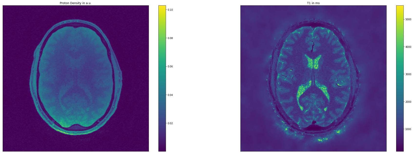
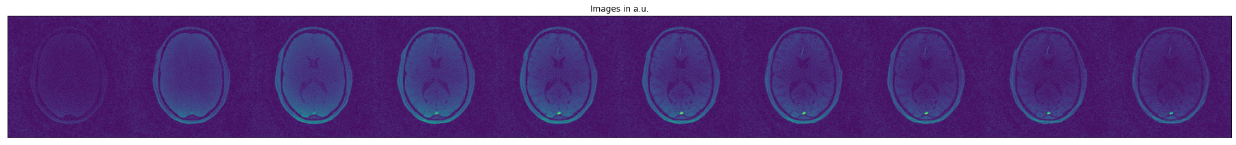
As final step, we can visualize the fitting results for this example (tgv_result_iter_6) and the initial images after CG-SENSE reconstruction:
[ ]:
with h5py.File('sample_data/PyQMRI_out/VFA/'+outdirs_VFA[-1]+os.sep+files[-1],'r') as file:
  result = file["tgv_result_iter_6"][()]
  images = file["images_ifft"][()]

%matplotlib inline

import matplotlib.pyplot as plt

num_images = images.shape[0]
images = np.swapaxes(images, -2, -1)
images = images.reshape(images.shape[-2]*num_images, -1).T
fig = plt.figure(figsize=(32,4))
ax = fig.add_subplot(111)
ax.get_xaxis().set_visible(False)
ax.get_yaxis().set_visible(False)
plt.imshow(np.abs(np.squeeze(images)))
plt.title('Images in a.u.')
plt.show()
[ ]:
fig = plt.figure(figsize=(32,11))
ax = fig.add_subplot(121)
ax.get_xaxis().set_visible(False)
ax.get_yaxis().set_visible(False)
M0_plot = plt.imshow(np.abs(np.squeeze(result[0])))
cb = plt.colorbar(M0_plot)
tmp = plt.title('Proton Density in a.u.')
ax = fig.add_subplot(122)
ax.get_xaxis().set_visible(False)
ax.get_yaxis().set_visible(False)
T1_plot = plt.imshow(np.abs(np.squeeze(result[1])))
cb = plt.colorbar(T1_plot)
tmp = plt.title('T1 in ms')